Solvency II aims to unify the EU insurance market and will come into effect on January 1st 2016. The technical specifications published by EIOPA will be used for interim reporting during 2015.
Although the specifications are not yet finalized, it is unlikely that they will change extensively. The technical specifications consist of two parts; part one focuses on the valuation and calculation of the capital requirements and part two focuses on the long-term guarantee (LTG) package. The LTG package was agreed upon in November 2013 and has been one of the key areas of debate in the Solvency II legislation.
Artificial volatility
The LTG package consists of regulatory measures to ensure that short-term market movements are appropriately treated with regards to the long-term nature of the insurance business. It aims to prevent ‘artificial’ volatility in the ‘own funds’ of insurers, while still reflecting the market consistent approach of Solvency II. When insurance companies invest long-term in fixed income markets, they are exposed to credit spread fluctuations not related to an increased probability of default of the counterparty.
These fluctuations impact the market value of the assets and own funds, but not the return of the investments itself as they are held to maturity. The LTG package consists of three options for insurers to deal with this so-called ‘artificial’ volatility: the Volatility Adjustment, the Matching Adjustment and transitional measures.
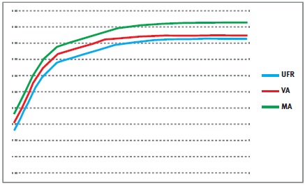
Figure 1
The transitional measures allow insurers to move smoothly from Solvency I to Solvency II and apply to the risk-free curve and technical provisions. However, the most interesting measures are the Volatility Adjustment and the Matching Adjustment. The impact of both measures is difficult to assess and it is a strategic choice which measure should be applied.
Both try to prevent fluctuations in the own funds due to artificial volatility, yet their requirements and use are rather different. To find out more about these differences, we immersed ourselves into the impact of the Volatility Adjustment and the Matching Adjustment.
The Volatility Adjustment
The Volatility Adjustment (VA) is a constant addition to the risk-free curve, which used to calculate the Ultimate Forward Rate (UFR). It is designed to protect insurers with long-term liabilities from the impact of volatility on the insurers’ solvency position. The VA is based on a risk-corrected spread on the assets in a reference portfolio. It is defined as the spread between the interest rate of the assets in the reference portfolio and the corresponding risk-free rate, minus the fundamental spread (which represents default or downgrade risk).
The VA is provided and updated by EIOPA and can differ for each major currency and country. The VA is added to the liquid part of the risk-free zero-coupon rates, i.e. until the so-called Last Liquid Point (LLP). After the LLP, the curve converges to the UFR. The resulting rates are used to produce the relevant risk-free curve.
The Matching Adjustment
The Matching Adjustment (MA) is a parallel shift applied to the entire basic risk-free term structure and serves the same purpose as the VA. The MA is calculated based on the match between the insurers’ assets and the liabilities. The MA is corrected for the fundamental spread. Note that, although the MA is usually higher than the VA, the MA can possibly become negative. The MA can only be applied to a portfolio of life insurance obligations with an assigned portfolio of assets that covers the best estimate of the liabilities.
The mismatch between the cash flows of the assets and the cash flows of the liabilities must not be a material risk in relation to the risks inherent to the insurance business. These portfolios need to be identified, organized and managed separately from other activities of the insurers. Furthermore, the assigned portfolio of assets cannot be used to cover losses arising from other activities of the insurers.
The more of these portfolios are created for an insurance company, the less diversification benefits are possible. Therefore, the MA does not necessarily lead to an overall benefit.
Differences between VA and MA
The main difference between the VA and the MA is that the VA is provided by EIOPA and based on a reference portfolio, while the MA is based on a portfolio of the insurance company.
Other differences include:
- The VA is applied until the LLP, after which the curve converges to the UFR, while the MA is a parallel shift of the whole risk-free curve;
- The MA can only be applied to specifically identified portfolios;
- The VA can be used together with the transitional measures in the preparatory phase, the MA cannot;
- The MA has to be taken into account for the calculation of the Solvency Capital Requirement (SCR) for spread risk. The VA does not respond to SCR shocks for spread risks.
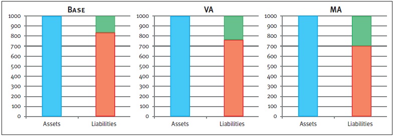
Figure 2: Graphical representations of balance sheets. The blue box represents the assets, the red box the liabilities, and the green box the available capital.
The impact of the VA and MA is twofold. Both adjustments have a direct impact on the available capital and next to this, the MA impacts the SCR. As a result, the level of free capital is affected as well. While the exact impact of the adjustments depends on firm-specific aspects (e.g. cash flows, the asset mix), an indication of the effects on available capital as well as the SCR is given in Figure 2. Please note that this is an example in which all numbers are fictitious and used merely for illustrative purposes.
Impact on available capital
Both the VA and the MA are an addition to the curve used to discount the liabilities, and will therefore lead to an increase in the available capital. The left chart in Figure 2 shows the Base scenario, without adjustment to the risk-free curve. Implementing the VA reduces the market value of the liabilities, but has no effect on the assets. As a result, the available capital increases, which can be seen in the middle chart.
A similar but larger effect can be seen in the right chart, which displays the outcome of the MA. The larger effect on the available capital after the MA compared to the VA is due to two components.
- The MA is usually higher than the VA, and
- the MA is applied to the whole curve.
Impact on the SCR
The calculation of the total SCR, using the Standard Formula, depends on several marginal SCRs. These marginal SCRs all represent a change in an associated risk factor (e.g. spread shocks, curve shifts), and can be seen as the decrease in available capital after an adverse scenario occurs. The risk factors can have an impact on assets, liabilities and available capital, and therefore on the required capital.
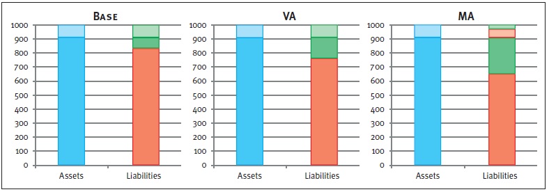
Take for example the marginal SCR for spread risk. A spread shock will have a direct, and equal, negative impact on the assets for each scenario. However, since a change in the assets has an impact on the level of the MA, the liabilities are impacted too when the MA is applied. The two left charts in Figure 3 show the results of an increase in the spread, where, by applying the spread shock, the available capital decreases by the same amount (denoted by the striped boxes).
Figure 3: Graphical representations of balance sheets after a positive spread shock. The lined boxes represent a decrease of the corresponding balance sheet item. Note that, in the MA case, the liabilities decrease (striped red box) due to an increase of the MA.
Hence, the marginal SCR for the spread shock will be equal for the Base case and the VA case. The right chart displays an equal effect on the assets. However, the decrease of the assets results in an increase of the MA. Therefore, the liabilities decrease in value too. Consequently, the available capital is reduced to a lesser extent compared to the Base or VA case.
The marginal SCR example for a spread shock clearly shows the difference in impact on the marginal SCR between the MA on the one hand, and the VA and Base case on the other hand. When looking at marginal SCRs driven by other risk factors, a similar effect will occur. Note that the total SCR is based on the marginal SCRs, including diversification effects. Therefore, the impact on the total SCR differs from the sum of the impacts on the marginal SCRs.
Impact on free capital
The impact on the level of free capital also becomes clear in Figure 3. Note that the level of free capital is calculated as available capital minus required capital. It follows directly that the application of either the VA or the MA will result in a higher level of free capital compared to the Base case. Both adjustments initially result in a higher level of available capital.
In addition, the MA may lead to a decrease in the SCR which has an extra positive impact on the free capital. The level of free capital is represented by the solid green boxes in Figure 3. This figure shows that the highest level of free capital is obtained for the MA, followed by the VA and the Base case respectively.
Conclusion
Our example shows that both the VA and the MA have a positive effect on the available capital. Apart from its restrictions and difficulties of the implementation, the MA leads to the greatest benefits in terms of available and free capital.
In addition, applying the MA could lead to a reduction of the SCR. However, the specific portfolio requirements, practical difficulties, lower diversification effects and the possibility of having a negative MA, could offset these benefits.
Besides this, the MA cannot be used in combination with the transitional measures. In order to assess the impact of both measures on the regulatory solvency position for an insurance company, an in-depth investigation is required where all firm specific characteristics are taken into account.